线性回归
线性回顾是最近基本的机器学习模型,它包含了机器最基本的思想。
- 确定学习模型和损失函数,初始化参数
- 损失函数的各个变量的梯度,根据学习步长产生新的变量
- 迭代步骤2,直到损失函数值不在缩小或者达到预定的迭代次数时, 退出循环,损失函数最小时,就是当前学习到的最优模型
准备实验数据
  %matplotlib inline
  import matplotlib.pyplot as plt
  import numpy as np


  plt.rcParams['font.sans-serif'] = ['SimHei'] # 指定默认字体
  plt.rcParams['axes.unicode_minus'] = False # 解决保存图像是负号'-'显示为方块的问题
# Out[10]:
x_data = [338., 333., 328., 207., 226., 25., 179., 60., 208., 606.]
y_data = [640., 633., 619., 393., 428., 27., 193., 66., 226., 1591.]
x_d = np.asarray(x_data)
y_d = np.asarray(y_data)
初始化模型
import time

x = np.arange(-200, -100, 1)
y = np.arange(-5, 5, 0.1)
Z = np.zeros((len(x), len(y)))
X, Y = np.meshgrid(x, y)

# loss
for i in range(len(x)):
    for j in range(len(y)):
	b = x[i]
	w = y[j]
	Z[j][i] = 0  # meshgrid吐出结果:y为行,x为列
	for n in range(len(x_data)):
	    Z[j][i] += (y_data[n] - b - w * x_data[n]) ** 2
	Z[j][i] /= len(x_data)


# linear regression
b = -120
w = 1.0

# 先人工利用先验知识 设置参数b, w的不同学习步长
lr = 0.00005
lrb = 1.0
iteration = 14000
训练迭代
b_history = [b]
w_history = [w]
loss_history = []
start = time.time()
for i in range(iteration):
    m = float(len(x_d))
    y_hat = w * x_d + b
    loss = np.dot(y_d - y_hat, y_d - y_hat) / m
    grad_b = -1.0 * np.sum(y_d - y_hat) / m
    grad_w = -1.0 * np.dot(y_d - y_hat, x_d) / m
    # update param
    b -= lrb * grad_b
    w -= lr * grad_w

    b_history.append(b)
    w_history.append(w)
    loss_history.append(loss)
    if i % 1000 == 0:
	print("Step %i, w: %0.4f, b: %.4f, Loss: %.4f" % (i, w, b, loss))

end = time.time()
print("大约需要时间:", end - start)
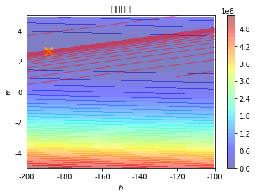
绘制学习曲线
# plot the figure


cp = plt.contourf(x, y, Z, 50, alpha=0.5, cmap=plt.get_cmap('jet'))  # 填充等高线
plt.plot([-188.4], [2.67], 'x', ms=12, mew=3, color="orange")
plt.plot(b_history, w_history, 'o-', ms=1, lw=1, alpha=0.5, color='red')

plt.xlim(-200, -100)
plt.ylim(-5, 5)
plt.xlabel(r'$b$')
plt.ylabel(r'$w$')
plt.title("线性回归")
plt.colorbar(cp)
plt.show()